1. Introduction
In this post, I would like to compare the loss functions used in different one-shot object detection methods, YOLO, SSD, and RetinaNet. One-shot object detection methods train the model on more than thousands grids with different scale, but the number of objects in one image is much less. The distribution of foreground (object) and background is extremely imbalanced. THe rest of the post is focused on the 3 different ways to overcome this problem.
2. YOLO
The loss function of YOLO is the sum of 5 parts as follows:
- $\lambda_{coord} \sum_{i=0}^{S^2} \sum^B_{j=0} \mathbb{1}_{ij}^{obj} [(x_i - \hat{x_i})^2 + (y_i - \hat{y_i})^2]$
- $\lambda_{coord} \sum_{i=0}^{S^2} \sum^B_{j=0} \mathbb{1}_{ij}^{obj} [(\sqrt{w_i} - \sqrt{\hat{w_i}})^2 + (\sqrt{h_i} - \sqrt{\hat{h_i}})^2]$
- $\sum_{i=0}^{S^2} \sum^B_{j=0} \mathbb{1}_{ij}^{obj} (C_i - \hat{C_i})^2$
- $\lambda_{noobj} \sum_{i=0}^{S^2} \sum^B_{j=0} \mathbb{1}_{ij}^{noobj} (C_i - \hat{C_i})^2$
- $\sum_{i=0}^{S^2} \sum_{c \in classes} \mathbb{1}_{i}^{obj} (p_i(c) - \hat{p_i}(c))^2$
where 1 and 2 are the loss for the regression of boxes, 3, 4, and 5 are the loss of classification.
Generally speaking, cross entropy is used as the loss function for classification. However, the square error is used in YOLO. As introduced by the authors, the square error is not stable for the training at the beginning, while it reaches a good performance in the end. In order to solve the problem of imbalanced data, a parameter $\lambda_{noobj}$ is added to lower the importance of the loss of no object grid.
3. SSD
In the model of SSD, the loss function for the classification is:
$L_{conf}(x,c) = - \sum^N_{i \in Pos} x_{ij}^p log(\hat{c_i^p}) - \sum_{i \in Neg} log(\hat{c_i^o})$
The confidence loss is the loss in making a class prediction. For every positive match prediction, we penalize the loss according to the confidence score of the corresponding class. For negative match predictions, we penalize the loss according to the confidence score of the class “0”: class “0” classifies no object is detected.
Hard negative mining: However, we make far more predictions than the number of objects presence. So there are much more negative matches than positive matches. This creates a class imbalance which hurts training. We are training the model to learn background space rather than detecting objects. However, SSD still requires negative sampling so it can learn what constitutes a bad prediction. So, instead of using all the negatives, we sort those negatives by their calculated confidence loss. SSD picks the negatives with the top loss and makes sure the ratio between the picked negatives and positives is at most 3:1. This leads to a faster and more stable training.
4. RetinaNet
RetinaNet introduces a new loss function, named focal loss (FL). The key idea of focal loss is: Our novel Focal Loss focuses training on a sparse set of hard examples and prevents the vast number of easy negatives from overwhelm- ing the detector during training.
$FL(p) = -(1-p)^{\gamma}log(p)$
The following image from the paper of RetinaNet shows the plot of focal loss with different parameter $\gamma$.
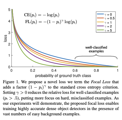
It’s easy to find the increasing of $\gamma$ adds increasing effort of lowering the importance of well classified example.
5. Conclusion
The common intuitive solution of the 3 models is to lower the importance of foreground loss. YOLO directly set small weights to foreground loss, SSD use part of the foreground to calculate the total loss, Retina considers the most of the foreground is easy to classify and use focal loss to reduce the importance of loss of the easy examples.