1. Introduction
In this post, I resume the development of Inception network from V1 to V4. The main purpose of this post is to clearly state the development of design of Inception network. For better understanding of the history, I list the time of the publication of the 4 paper and other important counterparts.
| Year | Inception Version | Other counterparts |
| 2014 | Inception V1[1] in Sept. | |
| 2015 | Inception V2[2] in Feb. | VGG[6] in Apr. |
| Inception V3[3] in Dec. | ResNet[5] in Dec. | |
| 2016 | Inception V4[4] in Feb. |
The versions of Inception are sometimes not agreed. Here I used the statement in the paper of Inception V4. The statement is as follows:
…GoogLeNet or Inception-v1 in our exposition. Later the Inception architecture was refined in various ways, first by the introduction of batch normalization (Inception-v2) by Ioffe et al. Later the architecture was improved by additional factorization ideas in the third iteration which will be referred to as Inception-v3 in this report.
So the versions of Inception in this post are defined as:
- Version 1[1] proposes the basic Inception network
- Version 2[2] proposes batch normalization
- Version 3[3] redesigns the network by factorizing the convolutional kernel
- Version 4[4] simplifies V3 with more uniform architecture and compares the performance with Inception-ResNet
In the rest of the post, each version of Inception Network is discussed in one section.
2. Inception V1
2-1. Principle of architecture design
As the name of the paper[1], Going deeper with convolutions, the main focus of Inception V1 is find an efficient deep neural network architecture for computer vision.
The most straightforward way to improving the performance of DNN is simply increase the depth and width. The main drawbacks of this method is the requirement of more data to overcome possible overfitting and more computational resource. The fundamental way to solve these 2 problem for computer vision system is to use sparsely connected architecture to replace the fully connected one.
I like the original words from paper[1]:
…if the probability distribution of the data-set is representable by a large, very sparse deep neural network, then the optimal network topology can be constructed layer by layer by analyzing the correlation statistics of the activations of the last layer and clustering neurons with highly correlated outputs. Although the strict mathematical proof requires very strong conditions, the fact that this statement resonates with the well known Hebbian principle – neurons that fire together, wire together – suggests that the underlying idea is applicable even under less strict conditions, in practice.
2-2. Detail of architecture design
2-2-1. Optimal local sparse structure
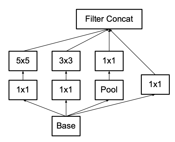
In the feature map, each unit can be considered as the representation of some region of input images. The 1$\times$1 convolutional kernel can encode this single region for the next layer. However, there are other features which are composed of more single regions. So the 3$\times$3 and 5$\times$5 convolutional kernel as well as maxpooling are used in parallel. All these features are stacked at the end of this layer. Image 1 shows an example:
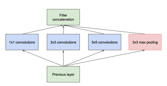
Image 1: Naive inception network
2-2-2. Dimension reduction
With the local structures introduced before, the computational cost is still very expensive. The author use dimension reduction by applying 1$\times$1 convotional kernel with less filters. Then feature maps are passed to 3$\times$3 and 5$\times$5 convolutional kernel.
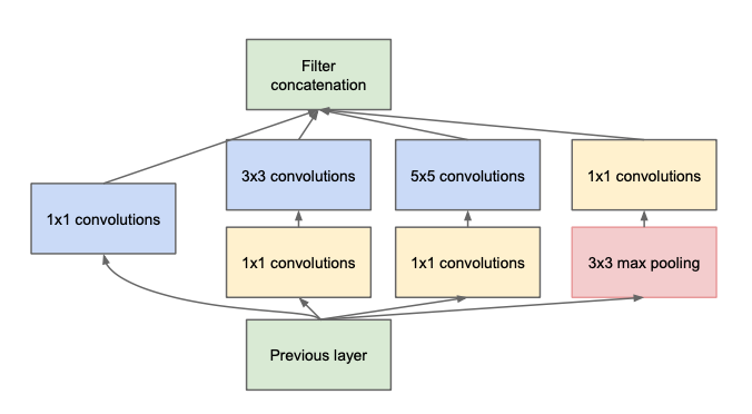
Image 2: Inception network with dimension reduction
2-3. Architecture
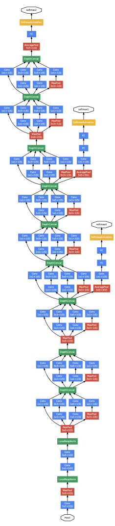
Image 3: Inception network architecture
3. Inception V2
The paper for Inception V2 is Batch normalization: Accelerating deep network training by reducing internal covariate shift. The most important contribution is introducing this normalization. As stated by the authors, Batch Normalization allows us to use much higher learning rates and be less careful about initialization. It also acts as a regularizer, in some cases eliminating the need for Dropout.
In Inception V2, the authors first propose the problem named Internal Covariate Shift (ICS). Then they suggest several solutions and analyse their advantage and drawbacks. The details are explained below.
3-1. Internal covariate shift
The change in the distribution of network activations due to the change in network parameters during training is defined as ICS. As inspired by the whitening technique for computer vision, we think the normalization to help training of the model. This is often performed to the input of the image. For example, the values of pixels of an image are normalized by subtracting the mean and being divided by the standard deviation.
Now, the question is can we do the same processing for all the internal input from layer to layer in a network.
- Possible solution 1: Suppose the normalization is independent to the optimization. But the experiments of this hypothesis shows that the model blows up, because the normalization is outside the gradient descent step.
- Possible solution 2: Take into account the normalization when doing gradient descent. However, the calculation cost is too high because of the computation of covariance matrix of all examples.
3-2. Normalization via Mini-Batch statistic
In order to reduce the computation, 2 simplifications are used:
- Normalize the layer inputs and outputs separately
- Use mini-batch statistics
For a layer with $d$-dimension input $x = (x^1, …, x^d)$, the normalization is as:
$\hat{x^k} = \frac{x^k - E[x^k]}{\sqrt{Var[x^k]}}$
But this normalization weakens the ability of representation. In order to have the possibility to revert or slight change this normalization, we add 2 parameters $\gamma^k$ and $\beta^k$, which are learned by the network.
$y^k = \gamma^k\hat{x^k} + \beta^k$
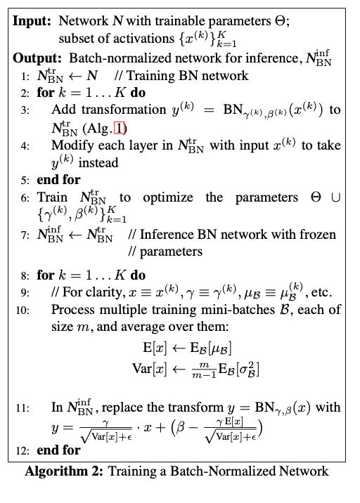
The algorithm of BN is shown below:
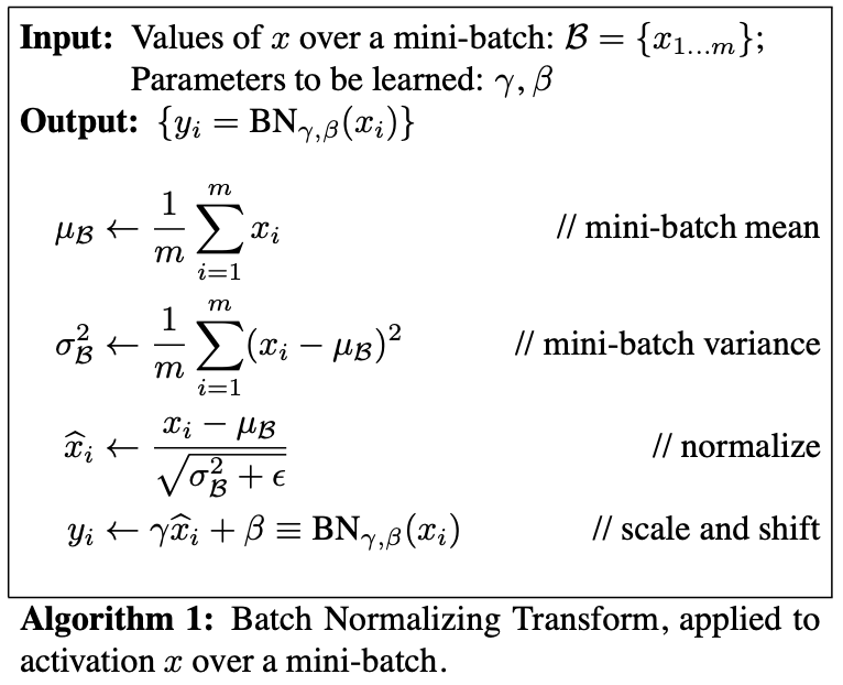
The full training and inference algorithm is as follows:
3-3. Main influence of BN
- Speed up the training process
- Stabilize the training
- Add regularization, so we can reduce other regularization(Dropout, less weight decay)
- BN needs more thoroughly shuffle
4. Inception V3
With version 1 and version 2, Inception have introduced sparse representation to reduce the calculation and batch normalization to speed up and stabilize the training. In version 3, the authors want to explore ways to scale up networks in ways that aim at utilizing the added computation as efficiently as possible by suitably factorized convolutions and aggressive regularization. They give some general design principles according to their large scale experimentation with various architectural.
- Avoid representational bottlenecks, especially early in the network.
- Higher dimensional representations are easier to pro- cess locally within a network.
- Spatial aggregation can be done over lower dimensional embeddings without much or any loss in representational power.
- Balance the width and depth of the network.
Let’s go into details.
4-2. Factorizing convolutions
The ideas mainly come from the discuss between added computation and benefits. For instance, the computation of a 5$\times$5 convolutional kernel is 26/9 = 2.78 times of the one of 3$\times$3 convolutional kernel. However, the similar results of applying 5$\times$5 convolutional kernel can be achieved by applying 2 times 3$\times$3 convolutional kernel. Meanwhile, the computation is less (9 + 9 < 25). In general, there are 2 kinds of factorization discussed in the paper.
4-2-1. Factorization into smaller convolutions
As discussed before, larger convolutional kernel can be replaced by several times of smaller kernels. In Inception V3, 5$\times$5 convolutional kernel is replace by 2 3$\times$3 convolutional kernel, shown in Image below:
Original with large kernel
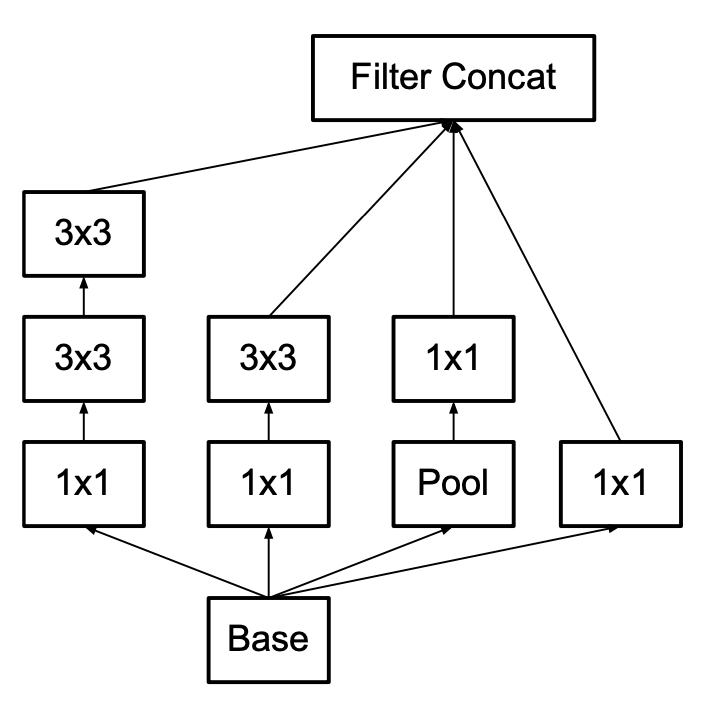
New with small kernel
4-2-2. Spatial Factorization into Asymmetric Convolutions
The authors indicate that one can replace any n × n convolution by a 1 × n convolution followed by a n × 1 convolution and the computational cost saving increases dramatically as n grows. Images below give an example:
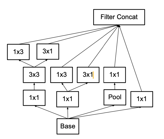
Original with symmetric kernel
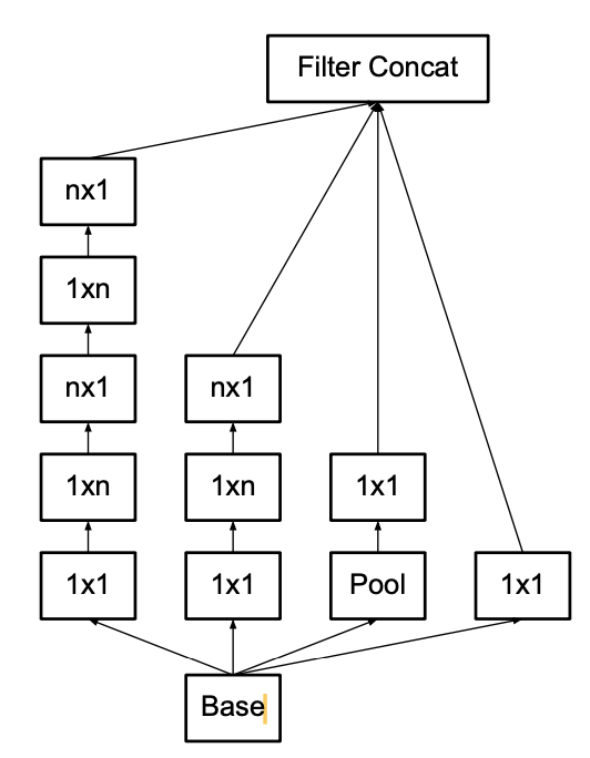
New with asymmetric kernel
4-3. Efficient grid size reduction
According to principle 1, it’s better to reduce the dimension latter. So we can use convolutional kernel with strides of 2 to reduce the dimension and do the convolution.
4-4. Label Smoothing
In cross entropy, the direct use the ground true to indicate the probability of certain class to 1 can cause 2 problems:
- causes overfitting
- encourages the differences between the largest logit and all others to become large, and this reduces the ability of the model to adapt.
The label smoothing can be simply understood as lower the probability of ground true from 1 to certain value, 0.9 for example.
4-5. Deal with low resolution image
One simple way to ensure constant effort is to reduce the strides of the first two layer in the case of lower resolution input, or by simply removing the first pooling layer of the network.
5. Inception V4
ResNet and Inception V3 get similar performance in image classification. So the authors want to check is the combination of these 2 structure can get better idea. Moreover, the authors want to check if Inception can be more efficient with deeper and wider structure.
Generally speaking:
- Inception-ResNet-v1: a hybrid Inception version that has a similar computational cost to Inception-v3
- Inception-ResNet-v2: a costlier hybrid Inception ver- sion with significantly improved recognition performance.
- Inception-v4: a pure Inception variant without residual connections with roughly the same recognition performance as Inception-ResNet-v2.
6. Conclusion
The key contribution of Inception Network:
- Filter the same region with different kernel, then concatenate all features
- Introduce bottleneck as dimension reduction to reduce the computation
- Introduce Batch Normalization
- Make network more efficient by using small kernel and asymmetric kernel
- Label smoothing
- Some important engineering experiences
- Inception-ResNet
Reference:
[1] Christian Szegedy, Wei Liu, Yangqing Jia, Pierre Sermanet, Scott Reed, Dragomir Anguelov, Dumitru Erhan, Vincent Vanhoucke, Andrew Rabinovich Going Deeper with Convolutions CVPR 2014
[2] Ioffe, Sergey and Szegedy, Christian Batch normalization: Accelerating deep network training by reducing internal covariate shift 2015
[3] Szegedy, Christian and Vanhoucke, Vincent and Ioffe, Sergey and Shlens, Jon and Wojna, Zbigniew Rethinking the inception architecture for computer vision CVPR 2015
[4] Szegedy, Christian and Ioffe, Sergey and Vanhoucke, Vincent and Alemi, Alexander A Inception-v4, inception-resnet and the impact of residual connections on learning AAAI 2016
[5] He, Kaiming and Zhang, Xiangyu and Ren, Shaoqing and Sun, Jian Deep residual learning for image recognition CVPR 2015
[6] He, Kaiming and Zhang, Xiangyu and Ren, Shaoqing and Sun, Jian Very deep convolutional networks for large-scale image recognition 2015