In this post, I would like to review the development of optimization methods for deep neural network (DNN) and share suggestions to use optimizers.
What you can find:
- A brief review of the popular optimizers from the an intuitive perspective.
- The disadavantage of the popular adaptive optimizer, Adam.
- Suggestions on jointly using different optimizers to achieve better performance.
Who may be interested:
- Want a brief overview of optimizers from SGD to Nadam.
- Want practices on how to use them.
1. Intuitive perspective of optimization
The goal of the optimization of DNN is to find the best parameters w to minimize the loss function $f(w, x, y)$, using $f(w)$ bellow for simplification, subject to $x, y$, where $x$ are the data and $y$ are the labels. The gradient descent (GD) is the most frequently used optimization method for machine learning. In this method, we need another parameter called learning rate, $\alpha$.
Now we start the process of gradient descent, at each batch/step t:
- Calculate the gradient of each parameter: $g_t = \bigtriangledown f(w_t)$
- Calculate the first order and/or second order momentum of gradient: $m_t=\phi(g_1, g_2, …, g_t)$ and $V_t = \psi(g_1^2, g_2^2, …, g_t^2)$
- Calculate the update value for w: $\eta_t = \alpha * m_t / (\sqrt{V_T} + \epsilon)$
- Update w: $w_{t+1} = w_t - \eta_t$
Next, let’s use these 4 steps to review different optimizers.
2. Review of optimizers
2-1. Batch gradient descent (BGD)
BGD calculates the gradients with entire training dataset for only one update of parameters. It can be very slow to converge. If the training dataset is too large to fill into the memory, BGD becomes intractable. Moreover, BGD is not compatible to update a model online, for example, with new data on-the-fly.
2-2. Stochastic gradient descent (SGD)
SGD calculates the gradients with one data. The calculation becomes faster, but the process of gradient descent becomes fluctuating. The direction of gradient descent calculated from only one data is not globally stable. It can be even opposite to the real gradient descent direction.
2-3. Mini-batch gradient descent
The trade-off between SGD and BGD is mini-batch gradient descent. This optimizer uses part of the data (n > 1) to calculate the gradients and update the parameters w. This is the most popular setup used in modern machine learning training process. In the rest of this story, SGD means SGD on mini-batch.
- Calculate the gradient of each parameter: $g_t = \bigtriangledown f(w_t)$
- Calculate the update value for w: $\eta_t = \alpha * g_t$
- Update $w$: $w_{t+1} = w_t - \eta_t$
2-4. SGD with momentum
Motivation: SGD has trouble in optimizing in ravine-like surface curves. It is easily blocked in the saddle point. Image 1[1] shows behaviors of different optimizers on a ravine-like curves at a saddle point. The final position of red point is called saddle point. Don’t worry about the new names in the image, I will introduce them in the rest of the story.
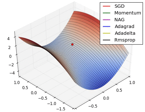
Image 1: Saddle point
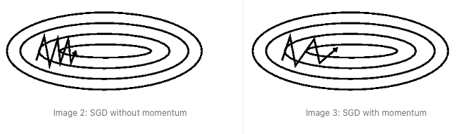
Image 2 and 3 [1] are the contour maps with local minimum in the middle. The lines with flash are the traces of optimization. For Image 2, it’s easy to find that the vertical step is big and horizontal step is small. But what we need is a big step along the horizontal direction and a small step along the vertical direction, which is depicted in the Image 3. The technique applied in Image 3 is call momentum, which accumulates the past gradients to determine current one to accelerate the convergence.
Solution: The implementation of SGD with momentum uses the method named exponential average. The exponential rate, $\beta$, is usually set to 0.9.
- Calculate the gradient of each parameter: $g_t = \bigtriangledown f(w_t)$
- Calculate the first order momentum of gradient: $m_t= \beta * m_{t-1} + \alpha * g_t$
- Calculate the update value for w: $\eta_t = m_t$
- Update $w$: $w_{t+1} = w_t - \eta_t$
2-5. SGD with Nesterov acceleration (Nesterov Accelerated Gradient, NAG)
Motivation: There are hundreds of thousands of parameters for a deep learning model. When we optimize the parameters in such a high dimension space, it’s easy to fall into a local minimum. If we can give the optimizer the ability to lookahead, it gives us more chance to step out the local minimum. SGD with Nesterov acceleration calculates the current gradients with a predicted approximation of w. The approximation is made by adding current w by the previous update value. Then the current update value is considered as a correction of the approximation. More explanations can be found in [2] and [3].
Solution:
- Calculate the gradient of each parameter: $g_t = \bigtriangledown f(w_t - \eta_{t-1})$
- Calculate the first order momentum of gradient: $m_t= \beta * m_{t-1} + \alpha * g_t$
- Calculate the update value for w: $\eta_t = m_t$
- Update $w$: $w_{t+1} = w_t - \eta_t$
2-6. AdaGrad
Motivation: The momentum give SGD the ability to adapt the update value according to the history of gradients. But the learning rate is the same for all parameters of w. Can we update the parameters with different learning rates depending on their importance? During the training of network, we can update slowly for those parameters associated with frequent features and update quickly for those parameters associated with infrequent features. So all the parameters can converge in similar rhythm. We use second order momentum to realize this proposition. We sum up the square of all past gradients of one parameter. The importance of this parameter is measured as dividing the general learning rate by the sum.
Solution:
- Calculate the gradient of each parameter: $g_t = \bigtriangledown f(w_t)$
- Calculate the second order momentum of gradient: $V_T = \sum_{t=1}^T g_t^2$
- Calculate the update value for w: $\eta_t = \alpha * g_t/ (\sqrt{V_T} + \epsilon)$
- Update $w$: $w_{t+1} = w_t - \eta_t$
2-7. AdaDelta/RMSprop
Motivation: The second order momentum calculated in AdaGrad is the accumulation of all the history, which becomes extremely big when the training process is long. This causes the update value infinitely close to 0 and the model can’t converge. In order to overcome this problem, we calculate exponential average of the second order momentum to replace the total accumulation of all past gradients.
Solution:
- Calculate the gradient of each parameter: $g_t = \bigtriangledown f(w_t)$
- Calculate the second order momentum of gradient: $V_t = \beta * V_{t-1} + (1-\beta) * g_t^2$
- Calculate the update value for w: $\eta_t = \alpha * g_t/ (\sqrt{V_t} + \epsilon)$
- Update $w$: $w_{t+1} = w_t - \eta_t$
2-8. Adam
Motivation: Adam is the most frequently used optimizer, since it combines the SGD with momentum and RMSProp. Solution:
- Calculate the gradient of each parameter: $g_t = \bigtriangledown f(w_t)$
- Calculate the second order momentum of gradient:
$m_t= \beta_1 * m_{t-1} + (1 - \beta_1) * g_t$
$V_t = \beta_2 * V_{t-1} + (1-\beta_2) * g_t^2$ - Calculate the update value for w: $\eta_t = \alpha * m_t/ (\sqrt{V_t} + \epsilon)$
- Update $w$: $w_{t+1} = w_t - \eta_t$
2-9. Nadam
Motivation: Does Adam combine all the methods talked before? It seems we forget Nesterov Accelerated Gradient. Let’s integrate it and this optimizer is called Nadam.
Solution:
- Calculate the gradient of each parameter: \$g_t = \bigtriangledown f(w_t - \alpha * m_{t-1}/ (\sqrt{V_{t-1}} + \epsilon)$
- Calculate the second order momentum of gradient:
$m_t= \beta_1 * m_{t-1} + (1 - \beta_1) * g_t$
$V_t = \beta_2 * V_{t-1} + (1-\beta_2) * g_t^2$ - Calculate the update value for w: $\eta_t = \alpha * m_t/ (\sqrt{V_t} + \epsilon)$
- Update $w$: $w_{t+1} = w_t - \eta_t$
Now, we have reviewed most of the optimizers for DNN with an intuitive perspective. Some practitioners consider the optimizers like Adam, SGD with momentum, etc. are the SGD with learning rate scheduler. My opinion is Yes and No. Scheduled learning rate can have the same effect as SGD with momentum, but it can’t update parameters with different learning rates.
3. Adam or SGD?
For new practitioners, it’s recommended to use Adam, which gives a good performance. Adam has an adaptive learning rate and is good at learning the representation of sparse data. But why lots of researchers still use SGD with momentum and with scheduled learning rate in their paper? What’s wrong with Adam? How can we use SGD with momentum to achieve better performance?
3-1. What’s wrong with Adam?
Problem 1: unconvergence
Paper [5] proves Adam could cause the unconvergence of the model in some case. Let’s check the details of the convergence when using different optimizers. In the method of SGD with first order momentum, the learning rate is fixed. When the model is converging, the update value becomes close to 0. For AdaDelta/RMSProp and Adam, the fluctuation of second order momentum can cause the unstable of the model. So the paper proposes to filter the second order momentum as follow:
$V_t = max(\beta_2 * V_{t-1} + (1-\beta_2) * g_t^2, V_{t-1})$
In this case, the update value shows a general decreasing tendency.
Problem 2: Local minimum
In the paper[6], the authors did experiments on CIFAR-10 database. Adam converges quicker than SGD, but the SGD has a better performance. Their conclusion is: The update value of Adam is too small to converge to global minimun at the end of training.
3-2. How to get better performance?
Adam and SGD, which one is better? It’s hard to say.
Although the convergence speed of Adam is high at the beginning of training, the experts prefer to use SGD or combine Adam and SGD because Adam may cause the model to be unstable or to converge to local minimum at the end of training. The authors of paper[6] recommend to use Adam at first for the quick convergence and use SGD to fine tune the model.
How can we combine Adam and SGD?
Let’s focus on the following 2 questions:
- When to switch from Adam to SGD?
- What learning rate should we use for SGD when switching from Adam?
Let’s first answer the second question. We recall the update value for SGD and Adam:
Adam: $\eta^{Adam}_t = \alpha^{Adam} * m_t / (\sqrt{V_t} + \epsilon)$
SGD: $\eta^{SGD}_t = \alpha^{SGD} * g_t$
We would like the SGD can at least update the parameters as Adam does. For this purpose, we project the Update Value of SGD ($UV_{SGD}$) to the direction of the update value of Adam ($UV_{ADAM}$). We have to ensure the projection of $UV_{SGD}$ on the direction of $UV_{ADAM}$ has the same value as $UV_{ADAM}$.
$proj(\eta^{SGD}) = \eta^{Adam}$
According to this equation, we can calculate learning rate α of SGD. The authors add exponential average filter to the learning rate for a more stable value, marked as $\lambda$. With the help of $\alpha$ and $\lambda$, let’s answer the first question: when to switch from Adam to SGD. As the authors mention in the paper, when the absolute difference between $\alpha$ and $\lambda$ is smaller than a threshold. It’s time to switch.
Reference:
- S. Ruder, An Overview of Gradient Descent Optimization Algorithm, https://ruder.io/optimizing-gradient-descent/index.html
- G. Hinton, N.Sricastava, K. Swersky, Nerual Networks for Machine Learning, http://www.cs.toronto.edu/~tijmen/csc321/slides/lecture_slides_lec6.pdf
- https://cs231n.github.io/neural-networks-3/#sgd
- https://zhuanlan.zhihu.com/p/32230623
- Sashank J. Reddi, Satyen Kale, Sanjiv Kumar, On the Convergence of Adam and Beyond, https://openreview.net/forum?id=ryQu7f-RZ
- Nitish Shirish Keskar, Richard Socher, Improving Generalization Performance by Switching from Adam to SGD, https://arxiv.org/abs/1712.07628