Review of YOLO: drawback and improvement from v1 to v3

1. Introduction

In this post, I’d like to review the 3 paper of YOLO. The main purpose is to understand the design of the YOLO and how the authors try to improve YOLO. For the details of implementation, such as learning rate and training tricks, please read the experiments parts in the paper[1][2][3]. This post is organized as:

1. The drawbacks of region proposal approach, as R-CNN, from the perspective of optimization
2. The design of YOLO V1
3. The drawbacks of previous version and improvement of current version of Yolo V2 and Yolo V3

2. Drawbacks of region proposal approach

Region proposal approach is also called 2-shot or 2-stage approach. The 2 steps are: propose regions which may contain objects and then do classification on proposed regions. As discussed in my previous post: Review of LeNet-5, a non-globally-trainable-system, as Region proposal approach, is hard to optimize because the individual module should be trained separately. In this post, I would like to analyse 2-shot approach from another point of view: optimization.

To perform a generic optimization, we check the 3 following aspects (BUD): bottleneck, unnecessary work, duplicated work. Let’s do the analysis for R-CNN, whose work flow is shown in Image 1[5].

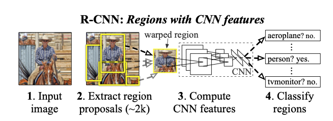
Image 1: Work flow of R-CNN

1. Bottleneck: R-CNN firstly (1) propose thousands of regions and then (2) do classification of object as well as regression to refine the bounding box on the proposed region. Since the classification and regression are repeated thousands times, there are lots of researchers focus on the optimization of (2).
2. Unnecessary work: I think there is no unnecessary work in the work flow of R-CNN.
3. Duplicated work: Too much duplicated work can be found in R-CNN. R-CNN use CNN to extract features for classification. There are 4 yellow rectangles in the step 2 in Image 1. Let’s focus on the 2 rectangles in the middle. We find that the higher one and the lower one share some overlapping region. The extraction of features on overlapping region is repeated 2 times.

What can we suggest to reduce the duplicated work? Let’s look at YOLO.

3. Design of YOLO V1

3-1. Unified detection

YOLO splits the image into $S*S$ grid cells, shown in Image 2[1].

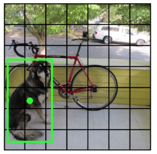
Image 2: Grid split

The regions of objects (the green rectangle) in the image are represented as a box. The center of the box (the green point) is defined as the center of an object. As the image is split into several grid cells, the center of an object falls into a grid cell. We consider this grid cell as the predictor, which predicts the class of object and the four corners of the box.

Each cell predict $B$ possible boxes. The prediction of each box includes the center point coordinates $x$ and $y$, the width $w$ and height $h$ of the box, and a probability to indicates how accurate the box is predicted.

The probability is defined formally as: $p(Object) * IOU_{pred.}^{truth}$.

where $p(Object)$ is the probability to have an object in the cell, $IOU_{pred.}^{truth}$ is the intersection over union between predicted region and the grand truth.

Moreover, every grid cell predicts conditional probabilities for $C$ types, marked as $p(Class_i|Object)$. To sum up, each grid predicts $B * 5 + C$ values and YOLO with $S*S$ cells predicts $S * S * (B * 5 + C)$ values.

Attention: each grid cell in YOLO V1 can predict only on object.

3-2. How to parametrize the predicted values?

The coordinates of box center, $x$ and $y$, are the offset to a particular grid cell and their values are between 0 and 1. The width $w$ and height $h$, are measured subject to the image width and height and their values are also between 0 and 1

3-3. The architecture of YOLO network

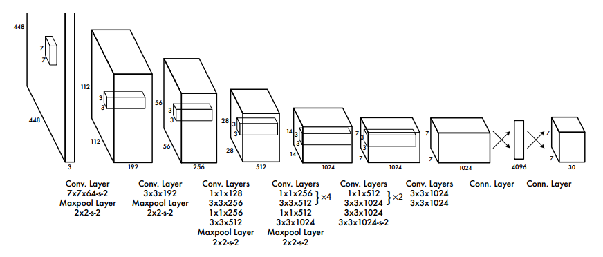
Image 3: The architecture of YOLO network

Image 3[1] shows clearly the architecture of YOLO. During the implementation, the last fully connected layer takes $4096$ vector as input and outputs a vector of $7*7*30$. Then we have to reshape it to a tensor with dimension of $7*7*30$.

In YOLO V1:

1. No Batch Normalization layer.
2. Activation function: LeakyReLU for all layers, except the last one, which uses linear activation.
3. Dropout: dropout layer with rate=0.5 after the first fully connected layer

3-4. Loss function

The loss function of YOLO is composed of the squared error of localization of box and classification and is the sum of the following 5 parts.

1. $\lambda_{coord} \sum_{i=0}^{S^2} \sum^B_{j=0} \mathbb{1}_{ij}^{obj} [(x_i - \hat{x_i})^2 + (y_i - \hat{y_i})^2]$
2. $\lambda_{coord} \sum_{i=0}^{S^2} \sum^B_{j=0} \mathbb{1}_{ij}^{obj} [(\sqrt{w_i} - \sqrt{\hat{w_i}})^2 + (\sqrt{h_i} - \sqrt{\hat{h_i}})^2]$
3. $\sum_{i=0}^{S^2} \sum^B_{j=0} \mathbb{1}_{ij}^{obj} (C_i - \hat{C_i})^2$
4. $\lambda_{noobj} \sum_{i=0}^{S^2} \sum^B_{j=0} \mathbb{1}_{ij}^{noobj} (C_i - \hat{C_i})^2$
5. $\sum_{i=0}^{S^2} \sum_{c \in classes} \mathbb{1}_{i}^{obj} (p_i(c) - \hat{p_i}(c))^2$

where $\mathbb{1}_{i}^{obj}$ denotes if object appears in cell $i$ and $\mathbb{1}_{i}^{obj}$ means the $j$th bounding box predictor in cell $i$ is in charge of the predicting. $\lambda_{coord}$ and $\lambda_{noobj}$ is used to remedy the problem of imbalanced data, because there are more cells without object than cells with objects. In the paper, $\lambda_{coord} = 5$ and $\lambda_{noobj} = 0.5$

In the part 2, the square root of width and height are used. Since the same prediction error of width and height has different influence for small box and large box, the square root can amplifier the influence when the box is small relate to large box. Do some calculation, you could find out this effect.

3-5. Benefits and drawbacks of YOLO V1

Benefits:

1. Fast
2. Global trainable system eases the optimization
3. More generalized, when testing on other database

Drawbacks:

1. Bad performance when there are groups of small objects, because each grid can only detect one object.
2. Main error of YOLO is from localization, because the ratio of bounding box is totally learned from data and YOLO makes error on the unusual ratio bounding box.

4. YOLO V2

In order to remedy the 2 problems mentioned before and improve the performance, the authors make several modifications in YOLO V2.

4-1. Batch Normalization

Adding Batch Normalization helps to improve mAP by 2%.

4-2. Hight Resolution classifier

YOLO V2 is trained on high resolution images for first 10 epochs. This improves the mAP by 4%

4-3. Convolutional with Anchor Boxes

One of the drawbacks of YOLO V1 is the bad performance in localization of boxes, because bounding boxes are learning totally from data. In YOLO V2, the authors add prior (anchor boxes) to help the localization. In order to introducing the anchors, some modifications are done on the architecture of the network.

1. Remove the fully connected layers
2. Shrink the input image dimension, so the feature maps after the final convolutional layers owns the same dimension as the grid. ($S*S$)
3. Move the prediction of the class of object from grid cell to bounding box. This means a cell can predict different objects with different boxes. So the prediction values for each box include 4 localization values for object, 1 confidence score for object, and $C$ conditional probabilities for class. In this case, every cell predicts $N * (C + 5)$, $N$ means the number of anchors used for one cell.

This improvement increases the recall value.

4-4.Dimension Clusters

This process decides the number of anchors and the predefined ratios for anchors.

4-5. Direct location prediction

The values of box center coordinates, $x$ and $y$, are between 0 and 1. But YOLO V1 can predict the values smaller than 0 or bigger than 1. The authors add logistic activation to force the prediction fall into the this range.

4-6. Fine-Grained Feature

This is a similar idea as feature pyramid. The authors reshape the last feature maps with 26 * 26 resolution to 13 * 13, and concatenate the reshaped feature maps to the output of last convolutional layer. The last convolutional layer outputs 13 * 13 * 1024 tensor. The reshaped feature map has dimension of 13 * 13 * 2048. The concatenating results has dimension of 13 * 13 * 3072.

4-7. Multi-scale Training

Training the model with images of different dimensions. The dimension of images are randomly chosen every 10 batch during the training.

4-8 New Architecture DarkNet-19

Image 4[2] shows the new architecture.

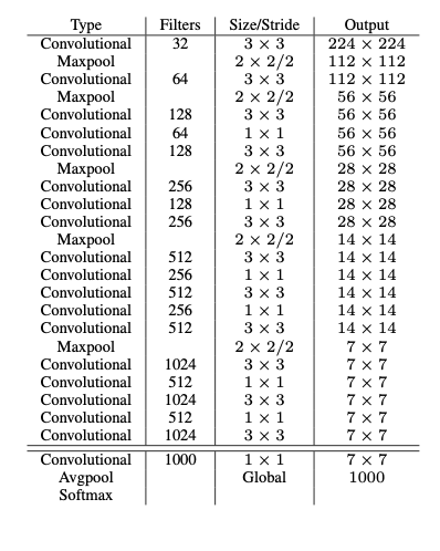
Image 4: The architecture of DarkNet-19

4-9. New mechanism

By introducing WordNet’s tree representation of object labels, YOLO V2 can train with data from different databases. This gives the YOLO the ability to predict about 9000 different objects. I think it’s not the improvement in the design of YOLO itself and this does not belong to the purpose of this post. Please check the paper for more information.

4-10. Conclusion of YOLO V2

Compared to YOLO V1, YOLO V2 becomes better, faster and stronger.

5. YOLO V3

The authors of YOLO have tried many technics to improve the accuracy and performance. Four of them work well for YOLO.

5-1. Bounding Box Prediction

YOLO V2 considers the confidence score as the multiplication of $p(Object)$ and $IOU(b, Object)$. First we calculate the probability of objectness, then take into account the IOU to adjust the probability. While YOLO V3 gives more intuitive understanding, which considers the confidence score of box directly as the probability of objectness. Then the probability of objectness is defined as the IOU of the predicted box and ground truth. By using logistic activation, the prediction is force to the range between 0 and 1.

5-2. Class Prediction

YOLO V2 uses softmax when calculating the conditional probabilities of classes. The softmax technique imposes the assumption that every box has only one label. But in reality, we often give object several labels, which can have overlapping. To solve the multi-label problem, YOLO V3 use independent logistic classification for each class. The binary cross-entropy is used to calculate the loss for each class.

5-3. Prediction Across Scales

YOLO V3 predict 3 boxes at each scale, so the tensor is $S * S * [3 * (4 + 1 + 80)]$. Unfortunately, the authors don’t indicate the detail information about how to calculate feature maps for the 3 scales. (I will write the details in my next post about the implementation of YOLOV3). In general, the 3 scales are:

1. Last convolutional layer, which has 32 stride compared to input dimension
2. The layer with 16 stride
3. The layer with 8 stride

If we have input images with dimension of 416 * 416, the 3 scales are in dimension of 13 * 13, 26 * 26, and 52 * 52.

5-4. New Architecture

The new architecture is named DarkNet-53, shown in Image 5[3].

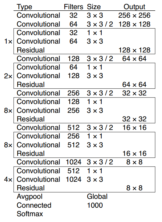
Image 5: The architecture of DarkNet-53

6. Conclusion

From YOLO V1 to YOLO V3, the authors showed us:

1. One-shot object detection
2. Move the prediction from cell to box to enable the detection of several objects in one cells
3. Use logistic activation for box prediction to constrain the range
4. Use logistic classification to enable multi-labeling
5. Use feature pyramid to reinforce the small object detection

Reference

[1] Joseph Redmon, Santosh Divvala, Ross Girshick, and Ali Farhadi   You Only Look Once: Unified, Real-Time Object Detection   CVPR 2016

[2] Joseph Redmon, Ali Farhadi   YOLO9000: Better, Faster, Stronger   CVPR 2017

[3] Joseph Redmon, Ali Farhadi   YOLOv3: An Incremental Improvement   Tech report

[4] Real-time Object Detection with YOLO, YOLOv2 and now YOLOv3

[5] Ross Girshick, Jeff Donahue, Trevor Darrell, Jitendra Malik   Rich feature hierarchies for accurate object detection and semantic segmentation   CVPR 2014